7. Results and Diagnostics
This chapter is the review pass after a completed project run. The recommended order is simple: confirm that the run finished cleanly, inspect the assimilation diagnostics, and only then interpret plots and compact output grids.
Most tutorial outputs live under:
/data/rofental/projects/project_2022_2023/
Because /data is a bind mount, open generated PNGs and the PDF with your normal
host applications under
<tutorial-workdir>/rofental/projects/project_2022_2023/results/. You do not need
an image viewer inside the container.
The most important locations are:
project_2022_2023.logresults/run_manifest.jsonresults/plots/perf/results/plots/assim/results/plots/results/results/maps/results/reports/results/misc/results/grids/da_output_grids.nc
1. Read the log first
Before interpreting plots, confirm that the run actually completed cleanly by checking the
end of project_2022_2023.log.
What to look for:
Project processing complete- data assimilation variable processing messages (
scf,wet_snow) - plot tasks completed
- data assimilation output summary NetCDF writing (
da_output_grids.nc) - setup cleanup and final run-manifest messages
If the log is not clean (important troubleshooting note)
If the log is not clean, treat downstream plots and tables as potentially incomplete or misleading.
Warning signs:
- repeated missing observation messages
- failures in a specific step
- plot task errors
- no data assimilation output export message
Advanced Troubleshooting (follow-up when the log shows errors)
2. Performance diagnostics (results/plots/perf)
The performance plots help you understand runtime distribution and resource behavior.
Files to inspect:
results/plots/perf/project_perf.pngresults/plots/perf/project_perf_metrics.csv
Reference structure snippet (results/plots/perf)
/data/rofental/projects/project_2022_2023/results/plots/perf/
  project_perf.png
  project_perf_metrics.csv
How to use these outputs:
- compare runtime across tutorial reruns
- estimate cost of increasing
ensemble_size- estimate cost of changing resolution (
100 mvs coarser)- identify unexpectedly slow stages (I/O, plotting, step-level hotspots)
Reference CSV snippet (performance metrics)
File path: /data/rofental/projects/project_2022_2023/results/plots/perf/project_perf_metrics.csv
| timestamp | cpu_total_pct | mem_used_pct | mem_used_gb | mem_total_gb | disk_fs_used_pct | disk_project_used_gb | cpu_temp_c | cpu_temp_source | thermal_sample_ok |
|---|---|---|---|---|---|---|---|---|---|
| 2026-02-21T21:28:14 | 0.00 | 4.10 | 1.01 | 24.45 | 30.10 | 0.82 | 48.2 | psutil:k10temp:Tctl | true |
| 2026-02-21T21:28:19 | 40.90 | 14.10 | 3.44 | 24.45 | 30.10 | 0.82 | 66.4 | psutil:k10temp:Tctl | true |
| 2026-02-21T21:28:24 | 53.30 | 16.00 | 3.91 | 24.45 | 30.11 | 0.82 | 72.8 | psutil:k10temp:Tctl | true |
| 2026-02-21T21:28:29 | 52.50 | 17.70 | 4.32 | 24.45 | 30.11 | 0.82 | 74.1 | psutil:k10temp:Tctl | true |
| 2026-02-21T21:28:34 | 61.90 | 19.40 | 4.74 | 24.45 | 30.11 | 0.82 | 76.0 | psutil:k10temp:Tctl | true |
The CSV also keeps absolute filesystem used/free/total columns (disk_fs_used_gb, disk_fs_free_gb, disk_fs_total_gb) and optional critical-temperature metadata. If thermal sensors are unavailable, cpu_temp_c and cpu_temp_crit_c are blank and thermal_sample_ok is false.
Plot file to open:
/data/rofental/projects/project_2022_2023/results/plots/perf/project_perf.png
Reference plot (tutorial baseline, ensemble_size=30):
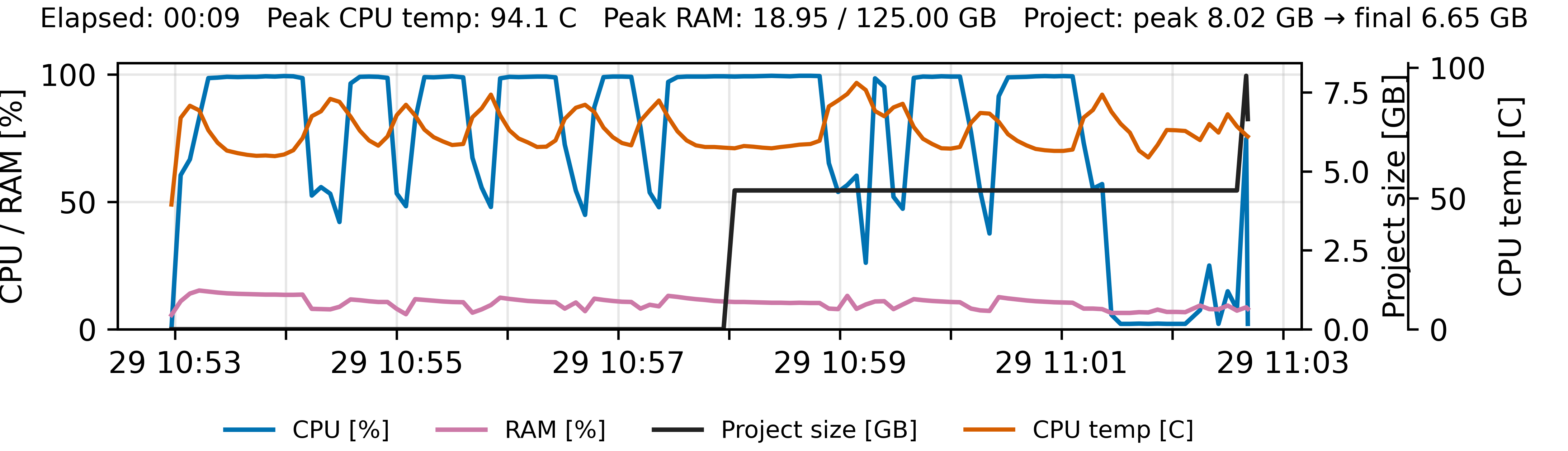
Approved clean v0.9.4 candidate telemetry from Lenovo P8 (100 m,
ensemble_size=30, 31 workers). Runtime and resource values are specific to
that machine.
What to read in the plot:
- Relative utilization curves: look for sustained CPU use during step processing and stable RAM use. Filesystem capacity telemetry remains in the CSV instead of competing with these curves in the figure.
- Project-size curve: follow project-directory growth across the steps. The final forced sample shows the drop after automatic restart-state cleanup; in this run, project size falls from an 8.02 GB peak to 6.65 GB. Live size comes from the storage reservation ledger after one baseline scan; the terminal point is reconciled against the physical tree.
- Thermal curve: when host sensors are readable, CPU temperature is plotted on its own axis. The heading reports p50/p95/maximum temperature and time above the configured reporting levels. These values do not by themselves prove thermal throttling.
- Timing structure: use
project_perf_phases.pngbeside the main plot to distinguish preflight, propagation, finalization and unmonitored restart gaps. Lines in the main plot break across such gaps rather than implying continuous sampling.
- Advanced Performance (deeper interpretation of runtime behavior)
3. Assimilation diagnostics (results/plots/assim)
These plots are the core data assimilation diagnostics.
Typical outputs:
results/plots/assim/weights/DA_XX_weights.pngresults/plots/assim/weights/setup_weights_overview_*.pngresults/plots/assim/ess/setup_ess_timeline_*.pngresults/plots/assim/scores/performance_scores.png
What they show:
- weights: how strongly observations favor some particles over others
- ESS (effective sample size): particle degeneracy indicator
- headline benchmark scores: update-date
CRPSS,NER, and station-onlyzSkillwhen available
Reference structure snippet (results/plots/assim, typical files)
/data/rofental/projects/project_2022_2023/results/plots/assim/
  ess/
    setup_ess_timeline_2022_2023.png
  scores/
    performance_scores.png
	weights/
	  DA_01_weights.png
	  ...
	  DA_08_weights.png
	  setup_weights_overview_2022_2023.png
    setup_weights_overview_2022_2023_page_02.png
    ...
Interpretation guidelines:
- ESS near ensemble size for many events:
- observations have weak discrimination or high observation error
- assimilation still updates the normalized PF weights; resampling was simply unnecessary
- ESS very low (near 1) frequently:
- strong degeneracy, aggressive resampling likely
- possibly too-small observation error (
obs_sigma) or too-strong mismatch- abrupt differences between station HS, fSCA, and wet-snow events:
- also normal and expected (different variables, support, and information content)
ESS is a diagnostic, not a simple “good/bad” score. Interpret it together with weights, variable type, and observation coverage.
Reference CSV snippet (weights for one station HS event)
File path: /data/rofental/projects/project_2022_2023/steps/step_04_20230131-20230221/assim/weights_station_hs_20230221.csv
| member_id | prior_weight | log_likelihood | weight | prior_ess | posterior_ess | resampled |
|---|---|---|---|---|---|---|
| member_001 | 0.00884 | -14.6988 | 0.00000000618 | 25.3132 | 14.6951 | true |
| member_002 | 0.04520 | -8.1494 | 0.00002208 | 25.3132 | 14.6951 | true |
Here weight is the normalized event posterior. When resampled is false, it
becomes the next step’s prior_weight; when true, resampled children start
uniformly.
Plot files to open:
/data/rofental/projects/project_2022_2023/results/plots/assim/ess/setup_ess_timeline_2022_2023.png/data/rofental/projects/project_2022_2023/results/plots/assim/scores/performance_scores.png/data/rofental/projects/project_2022_2023/results/plots/assim/weights/setup_weights_overview_2022_2023.png- if the setup has many assimilation dates, open the numbered continuation pages (
..._page_02.png,..._page_03.png, …) as well
- if the setup has many assimilation dates, open the numbered continuation pages (
/data/rofental/projects/project_2022_2023/results/plots/assim/weights/DA_04_weights.png
Reference ESS plot (tutorial baseline):
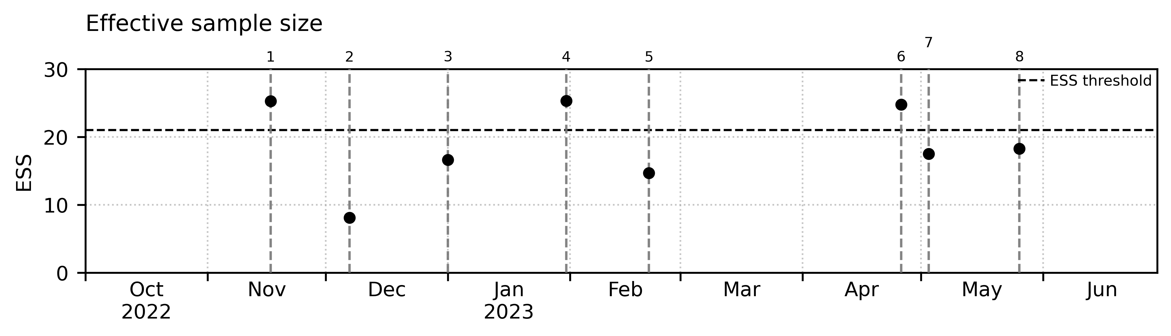
ESS timeline (setup_ess_timeline_2022_2023.png) from the tutorial reference
run. DA1, DA4 and DA6 remain above the threshold of 21 and therefore skip
resampling; the other events resample.
What to read in the ESS plot:
- each point corresponds to one assimilation event,
- lower ESS means stronger weight concentration (more degeneracy),
- differences between station HS, fSCA, and wet-snow events are expected because the observation types have different information content and spatial support.
Reference assimilation-date performance scores:
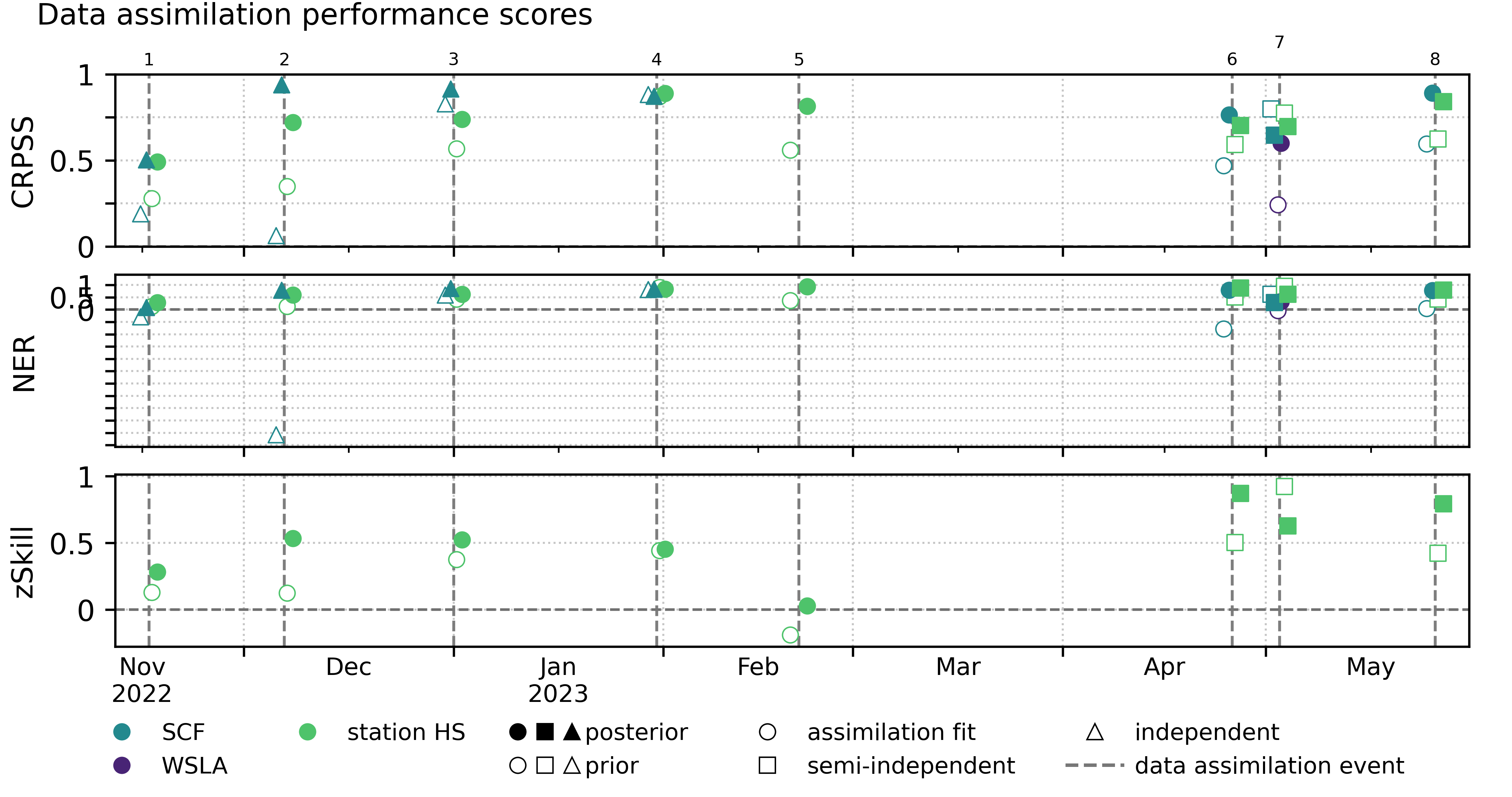
Prior and posterior CRPSS, NER and station-only zSkill for the configured assimilation dates. Use the benchmark tables for exact values and provenance.
This is an observation-based update diagnostic. It shows whether the weighted posterior improves relative to the prior for the evaluated observations, but it does not replace independent holdout validation.
Reference setup weights overview:
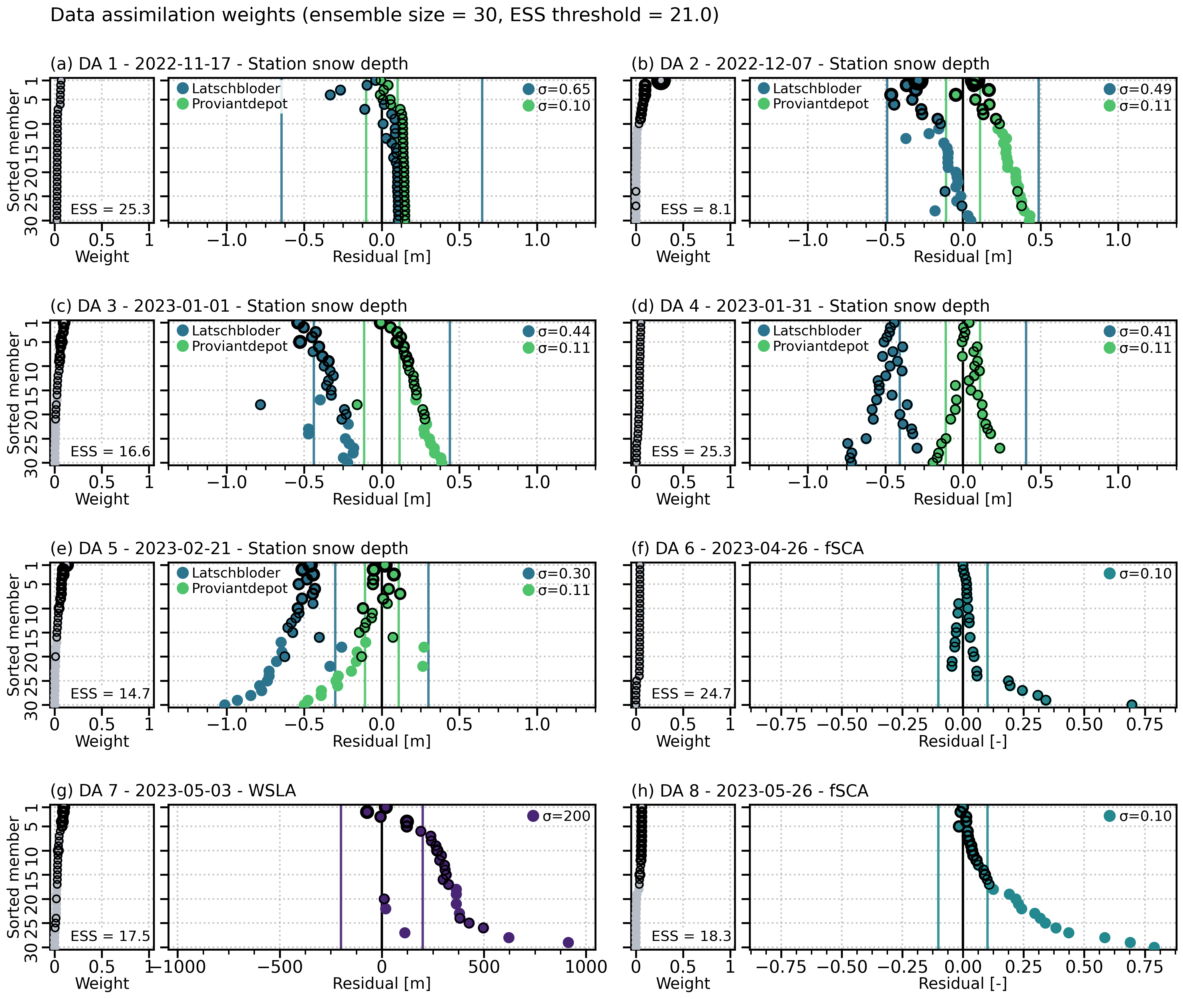
Setup-wide comparison of all eight assimilation events, grouped by observable family.
For larger projects, the setup overview is automatically split into multiple A4-length PNG pages that keep the first file name above and add numbered continuation pages.
Reference weights plot (example event):
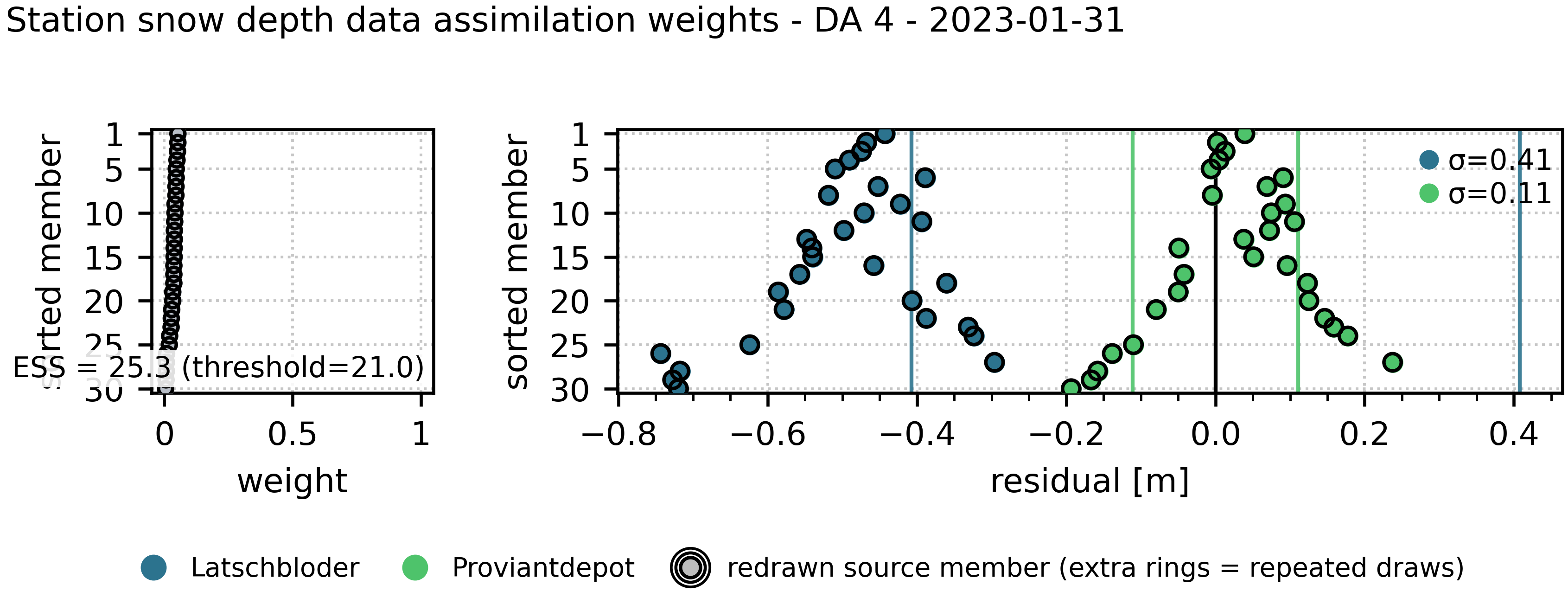
Weights plot for DA_04 (station_hs on 2023-02-21).
What to read in the weights plot:
- a flat distribution means the observation did not strongly discriminate particles,
- a peaked distribution means a few particles explain the observation much better,
- very strong peaks often coincide with low ESS and potential resampling pressure.
The weights overview uses one shared symmetric residual range per observable, based on the largest finite residual that is actually plotted. Events with many station-specific uncertainty values wrap their compact uncertainty key over multiple rows inside the panel.
With the tutorial’s fixed seeds and pinned release image, a run should reproduce the reference ensemble and diagnostics. Results can differ after changing the configuration, image, inputs or execution platform. For experiments, compare both the numeric outputs and the weight-distribution structure.
- Configuration Reference (likelihood, resampling, rejuvenation)
- Data Assimilation Methods (theory and terminology)
4. Point plots (results/plots/points)
This directory contains the stitched station and ROI point plots for the project.
Typical files include:
result_overview.png(configured high-level overview of observations, ensemble behavior, ESS and benchmark scores)- station snow depth plots
- station SWE plots
- ROI envelope exports and land-cover masking report
Reference structure snippet (results/plots/points, typical files)
/data/rofental/projects/project_2022_2023/results/plots/points/
  setup_results_point_latschbloder_snow_depth_2022_2023.png
  setup_results_point_proviantdepot_snow_depth_2022_2023.png
Result overview (high-level data assimilation behavior)
result_overview.png is often the fastest way to inspect:
- observation dates actually used,
- model-vs-observation fraction behavior,
- station snow-depth evolution relative to the open loop,
- ESS and assimilation-date score response,
- whether fSCA and wet-snow observations are present where expected.
The shipped Rofental project uses plots.yml to configure this standard overview. Other projects can use the built-in default panel list or provide their own panel order in the same file.
What to inspect:
- are observation markers present at the configured data assimilation dates?
- do fSCA and wet-snow events appear in the expected seasonal phases?
- are there obvious missing events or suspicious gaps?
Station plots
These plots support validation and interpretation of model behavior at observation stations.
When a matching station observation series is available, its line and the
station observation title qualifier are shown. Configured model points without
a matching observation series remain useful ensemble/open-loop diagnostics and
are labelled accordingly instead of claiming that an observation is present.
What to inspect:
- overall seasonal timing (accumulation / melt timing),
- amplitude differences (too much / too little snow),
- whether data assimilation shifts the ensemble envelope relative to the open loop,
- consistency across stations (important for tutorial interpretation).
Land-cover masking affects how much of the ROI contributes to fSCA/wet-snow summaries and fractions. This report is useful here because it explains the masking context behind the result plots and ROI envelope values shown in this chapter.
Reference CSV snippet (land-cover masking report)
File path: /data/rofental/projects/project_2022_2023/results/misc/lc_mask_report.csv
| class_code | class_name | cells | area_km2 | percent_of_roi |
|---|---|---|---|---|
| 2 | ice | 3257 | 32.57 | 32.82 |
| 3 | water | 15 | 0.15 | 0.15 |
| 10 | mixed forest | 48 | 0.48 | 0.48 |
| 8,9,10,11,12 | forest | 69 | 0.69 | 0.70 |
| total | total | 3346 | 33.46 | 33.72 |
How to use this table:
- confirm that excluded/retained classes look plausible for the tutorial ROI
- check whether
percent_of_roisuggests over-masking (unexpectedly little usable area) - use it as context when fSCA/wet-snow fractions look unexpectedly low/high
Recommended plot files to inspect (Rofental tutorial run):
/data/rofental/projects/project_2022_2023/results/plots/results/result_overview.png/data/rofental/projects/project_2022_2023/results/plots/points/setup_results_point_latschbloder_snow_depth_2022_2023.png/data/rofental/projects/project_2022_2023/results/plots/points/setup_results_point_proviantdepot_snow_depth_2022_2023.png
Suggested plot review order (practical)
result_overview.png(observation timing and availability)- ESS / weights plots (data assimilation behavior)
- Station plots
- NetCDF/grid outputs for spatial interpretation
Reference plots (tutorial baseline)
Result overview:
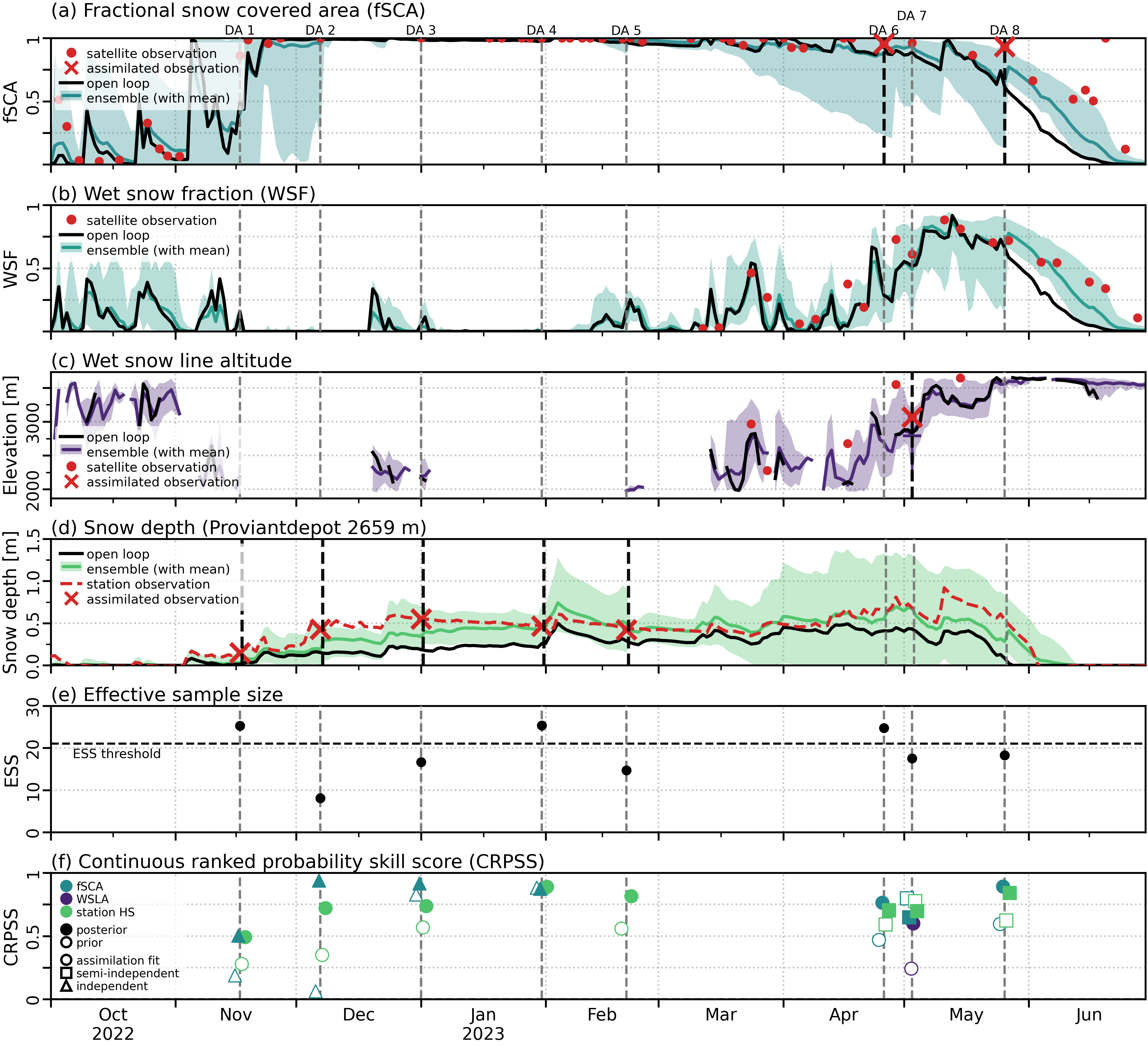
result_overview.png: check observation dates, fSCA/wet-snow event timing, station snow-depth behavior, ESS response and assimilation-date skill scores. Observations are red, with dashed station lines, satellite circles and X markers for assimilated observations.
What to read in this plot:
- whether observation markers exist at the configured data assimilation dates,
- whether fSCA events cluster in snow-cover relevant periods and wet-snow events in melt-season periods,
- whether the station snow-depth ensemble shifts away from or back toward the open loop during the season,
- whether ESS and CRPSS respond to the assimilation dates,
- whether data assimilation moves the ensemble envelope in the expected direction relative to the open loop.
Station snow depth example (latschbloder):
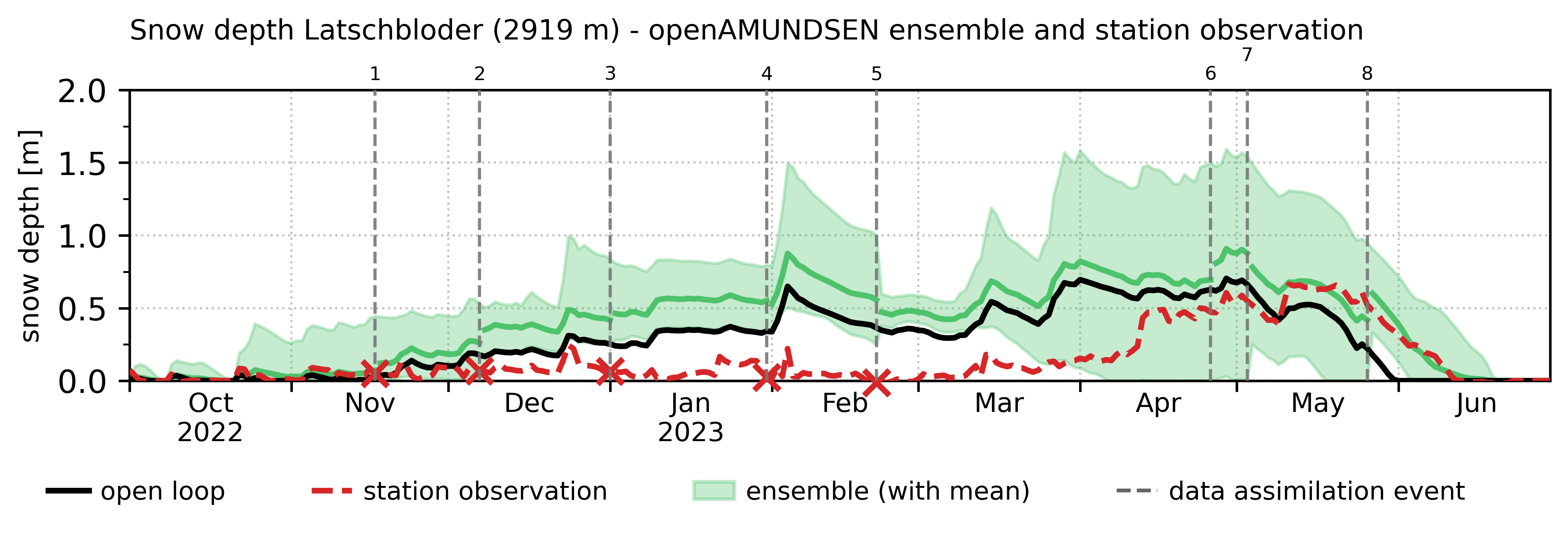
Snow depth comparison at latschbloder (open loop + ensemble + observations).
What to read in this plot:
- timing of snow accumulation and melt,
- whether observed values stay within (or near) the ensemble envelope,
- whether data assimilation visibly shifts the ensemble relative to the open loop around observation periods.
The shipped setup no longer applies a publication-only precipitation overlay. Its ensemble process noise comes directly from the project configuration shown in Chapter 6. This is a reproducible demonstration configuration, not a general tuning recommendation; see Example Data: Rofental.
More station reference plots (tutorial baseline)
proviantdepot snow depth:
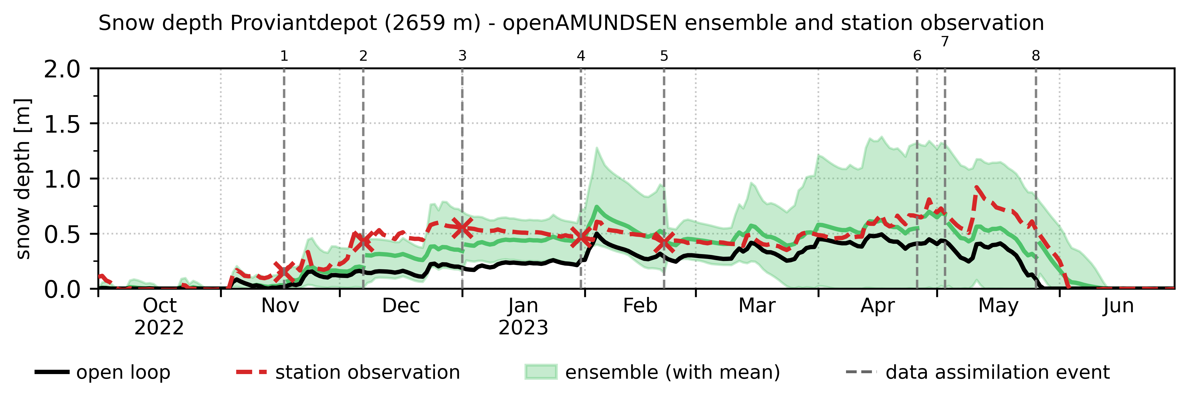
- Observation Processing (fSCA / wet-snow preprocessing context)
- Running the model (how the project lifecycle produces these plots)
5. data assimilation output summary NetCDF (da_output_grids.nc)
The tutorial setup writes a data assimilation output summary NetCDF:
results/grids/da_output_grids.nc
Output configuration (project YAML)
File path: /data/rofental/projects/project_2022_2023/project_2022_2023.yml
Relevant keys: data_assimilation.output.retention, data_assimilation.output.grids.format, data_assimilation.output.grids.variables[*]
This file is designed for:
- post-processing,
- visualization,
- comparison between runs,
- exporting selected variables in one merged file.
In the current tutorial configuration, data_assimilation.output.retention: full is enabled, so this summary NetCDF is written and the heavier member-grid artifacts are retained as well.
The summary NetCDF uses compact internal storage for data-assimilation-owned snow grids: snow depth is stored at 0.001 m resolution, while SWE and liquid-water content are stored at integer millimeter resolution. Normal CF-aware readers such as xarray return decoded physical values.
Reference output file path (data assimilation summary NetCDF):
/data/rofental/projects/project_2022_2023/results/grids/da_output_grids.nc
Optional variable/dimension inspection (Python in the container):
python - <<'PY'
import xarray as xr
ds = xr.open_dataset("/data/rofental/projects/project_2022_2023/results/grids/da_output_grids.nc")
print(ds)
print("\nVariables:")
for name in ds.data_vars:
    print("-", name, ds[name].dims)
PY
What to expect conceptually in the summary NetCDF:
- open-loop baseline fields
- ensemble mean / spread fields
- open-loop departure fields (
increment = ens_mean - open_loop)- assimilation-event analysis fields (
analysis_increment = analysis_mean - ens_mean) on event dates with weights
Dimension names in the inspected NetCDF (for example time1, time2, snow_layer, nbnd) are typically inherited from the underlying model outputs. Configure which variables/metrics are exported in the project YAML under data_assimilation.output.grids.variables[*]; see 6. Running the Model for the output-grid configuration note.
Raster output
Generated map examples from the Rofental tutorial reference run:
results/maps/da_events/da_7.png: WSLA update on 2023-05-03results/maps/da_events/da_8.png: fSCA (scf) update on 2023-05-26
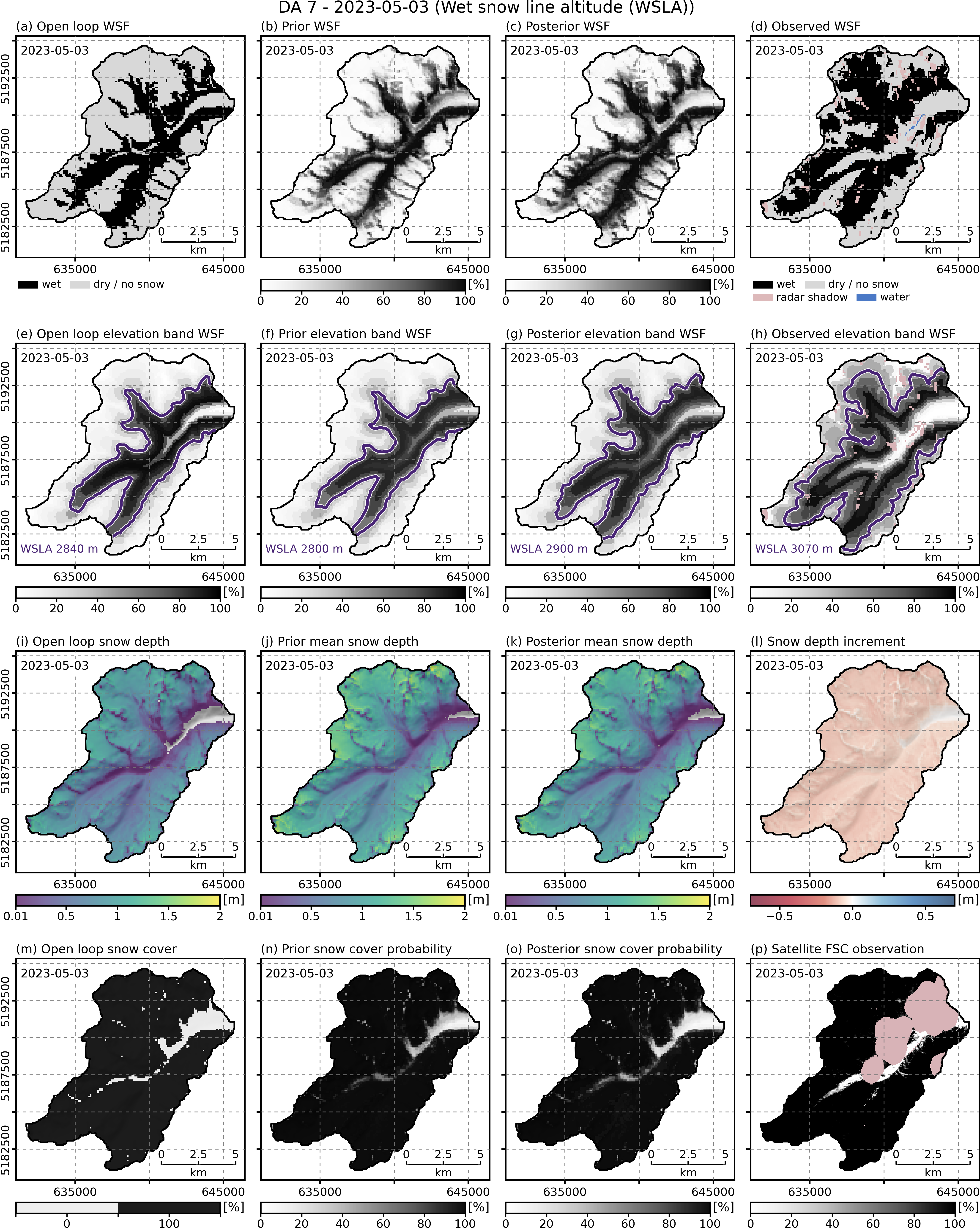
da_7.png: open loop, prior, posterior and observed wet snow fraction maps,
elevation-band wet snow fraction maps with the interpolated uppermost 50%
crossing, and corresponding snow-depth fields for the 2023-05-03
wet_snow_line update.
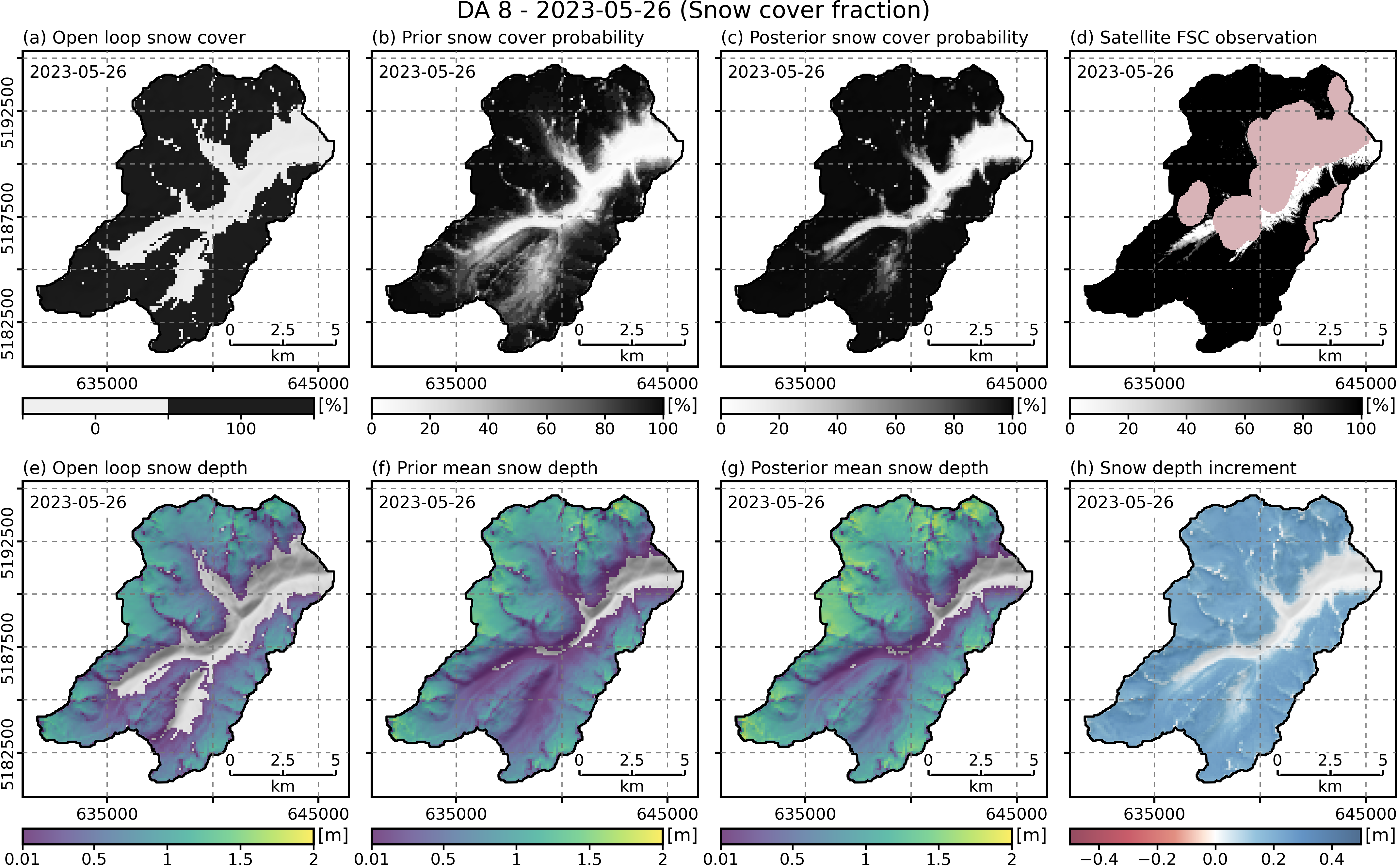
da_8.png: open loop, prior, posterior and observed fSCA diagnostics plus corresponding snow-depth fields for the 2023-05-26 scf update.
Note on raster workflow:
- all output grids are stored in one NetCDF file:
results/grids/da_output_grids.nc(see 5. data assimilation output summary NetCDF (da_output_grids.nc))- generated assimilation-event maps use event dates with available particle-filter weights
- for non-event dates, extract the layers/time slices you need in the GIS tool of your choice before styling or export
Reference snippet (NetCDF inspection, tutorial reference run):
dims: {'time2': 272, 'snow_layer': 3, 'y': 150, 'x': 160, 'time1': 273, 'nbnd': 2}
vars:
  ens_max_liquid_water_content
  ens_max_snowdepth_daily
  ens_max_swe_daily
  ens_mean_liquid_water_content
  ens_mean_snowdepth_daily
  ens_mean_swe_daily
  ens_min_liquid_water_content
  ens_min_snowdepth_daily
  ens_min_swe_daily
  ens_std_liquid_water_content
  ens_std_snowdepth_daily
  ens_std_swe_daily
  analysis_increment_liquid_water_content
  analysis_increment_snowdepth_daily
  analysis_increment_swe_daily
  analysis_mean_liquid_water_content
  analysis_mean_snowdepth_daily
  analysis_mean_swe_daily
  increment_liquid_water_content
  increment_snowdepth_daily
  increment_swe_daily
  open_loop_liquid_water_content
  open_loop_snowdepth_daily
  open_loop_swe_daily
Use results/grids/da_output_grids.nc in a GIS software of your choice and visualize raster output.
Recommended manual map date(s): choose one date with active snow cover and one date near melt season.
Use the same date across open_loop, ens_mean, and increment maps. Generated assimilation-event maps use four columns: open loop, prior, posterior, and reference. Snow depth maps use ens_mean as the prior mean, analysis_mean as the event-weighted posterior mean, and analysis_increment as posterior - prior.
For the shipped example, project maps are split into generated assimilation-event maps under results/maps/da_events/ and custom YAML maps such as setup_overview at the root of results/maps/. After changing plot or map configuration, optionally regenerate the complete configured presentation layer. Replace <MAX_WORKERS> with the worker limit chosen for the container; do not type the angle brackets.
openamundsen-da render \
  /data/rofental/projects/project_2022_2023 \
  --max-workers <MAX_WORKERS>
Omit --max-workers to let the container select the worker count from the visible
CPUs. Rendering validates and refreshes the configured plots, maps and project
report as one output set.
For snowdepth_daily, the map renderer uses the viridis palette together with a shared linear legend scale per render run. Tick labels are shown in cm, cells below 1 cm stay transparent so only meaningful snow cover is colored, and the top of the snow-depth legend is derived from the plotted maps. Increment panels use a signed red-blue diverging palette: negative increments are red, positive increments are blue. In generated assimilation-event maps, positive analysis_increment means the assimilation event added snow; negative means it removed snow.
A successful project run requires results/reports/project_report.pdf after the
plots, maps and benchmark outputs have validated. Use openamundsen-da render to
regenerate that complete configured output set after a presentation-only change.
The first PDF page summarizes the setup, wet-snow and liquid-water-content settings,
assimilation-event counts and computing-cost statistics. The remaining pages collect
the configured overview plots, maps and diagnostics in a compact review artifact.
data assimilation increment map
The tutorial includes generated assimilation-event maps above. For event-level diagnostics, use these maps or export
analysis_increment_snowdepth_daily from da_output_grids.nc on an assimilation date and compare it against the same-date prior/posterior mean maps.
- Configuration Reference (data assimilation output variable selection and metrics)
- Output data (where project outputs live)
- Data Assimilation Methods (how to interpret increments conceptually)
6. ROI envelopes and summary CSVs
The project now writes these setup-level envelope time series under results/misc/:
point_scf_roi_envelope.csvpoint_wet_snow_roi_envelope.csv
These summarize the ensemble spread over the ROI (mean, finite-member min-max range and sample count).
These CSVs are lightweight outputs that are ideal for quick comparisons between runs without loading NetCDF files.
Reference file paths for ROI envelope outputs:
/data/rofental/projects/project_2022_2023/results/misc/point_scf_roi_envelope.csv/data/rofental/projects/project_2022_2023/results/misc/point_wet_snow_roi_envelope.csv
Why these CSVs are useful:
- quick numeric QA without opening plots
- useful for external plotting notebooks or reports
- easy comparison across experimental runs
Reference CSV snippet (fSCA ROI envelope)
File path: /data/rofental/projects/project_2022_2023/results/misc/point_scf_roi_envelope.csv
| date | value_mean | value_min | value_max | n |
|---|---|---|---|---|
| 2022-10-01 | 0.00 | 0.00 | 0.00 | 11 |
| 2022-10-02 | 0.12 | 0.00 | 0.50 | 11 |
| 2022-10-03 | 0.08 | 0.00 | 0.40 | 11 |
| 2022-10-04 | 0.09 | 0.00 | 0.42 | 11 |
Reference CSV snippet (wet-snow ROI envelope)
File path: /data/rofental/projects/project_2022_2023/results/misc/point_wet_snow_roi_envelope.csv
| date | value_mean | value_min | value_max | n |
|---|---|---|---|---|
| 2022-10-01 | 0.00 | 0.00 | 0.00 | 11 |
| 2022-10-02 | 0.59 | 0.45 | 0.77 | 11 |
| 2022-10-03 | 0.04 | 0.00 | 0.14 | 11 |
| 2022-10-04 | 0.10 | 0.00 | 0.36 | 11 |
Interpretation:
value_mean: ensemble mean over finite ensemble membersvalue_min/value_max: finite-member minimum and maximumn: number of contributing ensemble members
7. Quick data assimilation sanity checklist (practical review routine)
Use this checklist as a quick review before trusting or comparing results.
Use this checklist after each tutorial run:
- Log ends with
Project processing completeresults/plots/perf/project_perf.pngexistsresults/plots/assim/contains ESS, weight, and score plotsresults/plots/results/result_overview.pngexists- Station plots exist (snow depth and SWE)
results/misc/point_scf_roi_envelope.csvandresults/misc/point_wet_snow_roi_envelope.csvexistresults/grids/da_output_grids.ncexists and opensIf one of these fails, check the log before changing configuration.
8. Project cleanup
After a successful single-domain project, openAMUNDSEN-DA automatically removes package-owned restart state files that are no longer needed. Cleanup happens only after the compact grid output, benchmark, plots, maps and report pass their checks. Failed and interrupted projects keep restart state so they can resume.
The scientific results remain available under
results/. Member grids are retained. Only restart state pickles and stale state pointers are eligible for automatic cleanup.
The successful project pipeline has already applied this cleanup. The commands below are the optional manual workflow for an older or incomplete project. First preview the eligible files:
openamundsen-da clean \
  /data/rofental/projects/project_2022_2023
Apply the preview only after checking it:
openamundsen-da clean \
  /data/rofental/projects/project_2022_2023 \
  --apply
Immediately after a successful tutorial run, preview: and applied: with no
listed files is the expected no-op result: there is no restart state left for the
manual command to remove.
What is removed:
- restart state pickle files under member
results/directories, - stale state pointers whose target no longer exists or is being removed.
- Output data (retention and cleanup contract)